Two sources of natural history information that I use often are the allaboutbirds.org and birdsoftheworld.org databases, both managed by Cornell’s Lab of Ornithology and both based on the exhaustive Handbook of the Birds of the World. These online databases contain a valuable trove of natural history information, but extracting the data into a format usable for quantitative applications is not straightforward.
One solution to this problem is html web scraping, and the purpose of this post is to provide a very brief overview of some simple web scraping packages in R and how to use them. This seemed especially useful to do since there are really not many online tutorials for web scraping ecological information from textual databases that I could find.
It would seem like simply downloading the full html text and calling various regular expressions would be the easiest way to approach this problem. And this might be true for very simple applications. But using this approach requires complex coding with a lot of if/else statements, is prone to errors, and doesn’t utilize the structured nature of the underlying html code. Fortunately, with some basic understanding of how html is structured and formatted, extracting any piece of information you want from an online data source is relatively simple and repeatable.
To begin, we’re going to extract some basic life history data for the Painted Bunting from allaboutbirds.org. Information about this species can be access freely from https://www.allaboutbirds.org/guide/Painted_Bunting/. The page looks something like this:
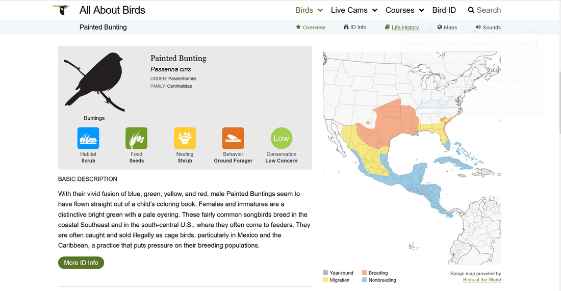
In the gray summary box you can find important information regarding the species preferred habitat, feeding preferences, and conservation status, etc. The steps below describe how to quickly and accurately extract this information and save it in a usable format.
Step 1: Loading html text into R
To start, we need to access the html text and load it into R. There are several functions that will do this, one of which is the ‘read_html’ function in the rvest package.
>library(rvest)
>bunting_html<-read_html(‘https://www.allaboutbirds.org/guide/Painted_Bunting/’)
Step 2: Identifying relevant html nodes
The trick to web scraping is understanding how the html data is structured using elements and node sets. Fortunately, you don’t really need to know all that much about html to perform simple web scrapes, but reviewing the basics is certainly helpful. The most important thing to understand is that the html data are organized in a very hierarchical and predictable structure. More specifically, there consists a series of headings, sub-headings, and associated content in the form of text, graphics, and whatever elements are found within the webpage.
To visualize this architecture, you can use the inspect function in your web browser. I am using firefox below, and this is accomplished by right clicking anywhere within the body of the web page.
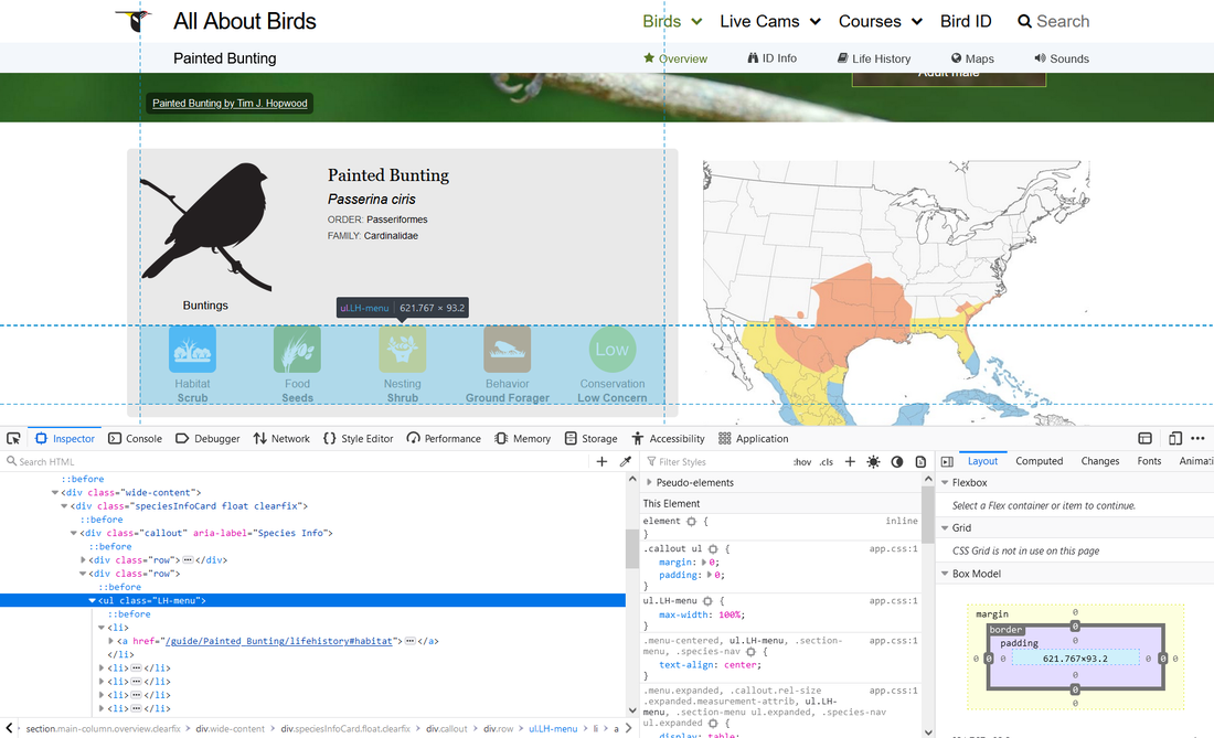
You will also notice that moving your cursor to various lines in the inspector tool will automatically highlight the relevant areas of the webpage that are generated from that line particular of code. This feature is very helpful for identifying which sections of the html code you need to access to get the data that you’re looking for. Similarly, where you right-click within the webpage to pull up the inspector tool will automatically highlight the associated hotml node set.
The section we are interested in is identified by the line <ul class=”LH-menu”>, which is highlighted in blue in the above image. If you hover over this line, it will highlight the section in the gray box that contains the five life history datapoints that we are interested in scraping.
We need the name of this node to access it in R. The name of a node is not always obvious. We know that it is a ‘ul’ node, but we don’t actually want all of the ‘ul’ nodes that are present in this url. We only want the specific node that is associated with the highlighted portion of the webpage. To get the name, simply right click on the appropriate line in the inspector tool, and select 'Copy CSS selector.' Again, this may be slightly different if you are using a different web browser, but it should be very similar.
Paste this somewhere, and we can see that the name of the node is ‘.LH-menu.’
Step 3: Accessing the relevant information
We will also use the rvest package to parse specific elemenets of the html data. Use of the rvest package requires some familiarity with pipes via the ‘%>%’ operator. If you have used the stringr package you will likely already be familiar with this.
To get the data from the .LH-menu node, we use the 'html_nodes' function:
>bunting_data<-bunting_html %>% html_nodes('.LH-menu')
This returns all of the content associated with the five life history categories shown above.
This, however, is a bit more information than we need. By doing some searching within the inspector tool, we can see that the data that we want (i.e., the five life history categories shown in the gray box above) are available within the 'img' sub-nodes. Accessing sub-nodes is done the same as above:
>bunting_data2<- bunting_data %>% html_nodes('img')
which returns:
{xml_nodeset (5)}
[1] <img src="/guide/images/icons/icon-scrub.png" alt="Habitat Scrub">
[2] <img src="/guide/images/icons/icon-seeds.png" alt="Food Seeds">
[3] <img src="/guide/images/icons/icon-shrub.png" alt="Nesting Shrub">
[4] <img src="/guide/images/icons/icon-ground-forager.png" alt="Behavior Ground Forager">
[5] <img src="/guide/images/icons/icon-low-concern.png" alt="Conservation Low Concern">
The data we are interested in are seen in parentheses on the right hand side of each line.
And this basically gets us all the way there. Figuring out the correct nodes to call is the biggest challenge with web scraping. Every situation will be different, and will likely require some tinkering and trial and error. Using the inspector tool in your web browser will help you identify the sections, node names, and relevant text that you need.
At this point, we could just extract the relevant text in each of the five nodes present in bunting_data using gsub or str_extract from the stringr package. For example:
> str_extract_all(word(as.character(bunting_data[1]), sep="alt=", -1), '\\w+')
returns:
[[1]]
[1] "Habitat" "Scrub"
But we can also do this more directly by identifying values of different attributes found within the nodes themselves. In the bunting_data object, each node contains two attributes: ‘src’ and ‘alt’, with the 'alt' attribute containging the life history information we are after.
Accessing attributes requires the xml2 package (other packages exist as well). To get the value of the 'alt' attribute, we use:
>bunting_data2<-xml_attr(bunting_data, 'alt')
We then remove the category names using str_split in the stringr package:
>bunting_data_3<- str_split(bunting_data2, " ")
>bunting_data_final<-lapply(bunting_data_3, function(x){paste[-1, collapse=“ ”})
Bunting_data_final returns a list of length five, indicating each of the life history categories we are looking for.
Step 4: Automating across multiple urls/species
Of course, going through the above steps takes much longer than simply looking at the webpage and transfering the data we want into excel. In most cases, though, we wish to access the same information for multiple species, or for all of the species in North American or even the globe.
For allaboutbirds.org, iterating over species is quite straightforward because of how the urls are structured. Specifically, species pages are identified using common names separated by an underscore. As such, a list of common names can be used to do something like:
>SpeciesList<-c(‘Painted_Bunting’, ‘American_Robin’, ‘Blue_Jay’, ‘American_Crow’)
>html_data<-vector(length=length(SpeciesList), mode=”list”)
>for(i in length(SpeciesList)){
> web_data<- paste("https://www.allaboutbirds.org/guide/", speciesList[i], sep="")
> html_data[[i]]<-read_html(web_data) ## modify this last part based on your needs
>}
Accessing multiple pages is more difficult for birdsoftheworld.org because the individual species pages are referenced using unique six letter codes. To access multiple pages, we need to know these codes, but from what I can tell, they are unique to birdsoftheworld.org, as I was unable to find them from any other source. Fortunately, we can scrape the codes directly from the website:
>species_page<-read_html(‘https://birdsoftheworld.org/bow/specieslist’)
>taxonomyNodes<- species_page %>% html_nodes('a')
>taxonomyNodes_codes<-taxonomyNodes %>% html_attr('href')
>BOW_codes<-lapply(taxonomyNodes_codes, function(x){str_match(x, '/bow/species/(.*?)/cur/introduction')[,2]})
>BOW_codes<-unlist(BOW_codes)
With the BOW_codes in hand, the individual species pages can be easily accessed.
Final Note
The birdsoftheworld.org pages contain much more information on most species than does allaboutbirds.org. Furthermore, the information present in each species page is more variable, including how the page content is structured. I mention this because in my experience, scraping data from birdsoftheworld.org is much more prone to errors. One solution is to add a TryCatch call to the loop. This useful function prevents termination of the loop when an error occurs for a particular species (e.g., if data are missing or the url turns out to be wrong). Something along the lines of:
>tryCatch(suppressWarnings(scrape_function, error = function(e) NA)
where scrape_function represents the specific task that you are trying to perform.
In addition to TryCatch, you may also need to include one or more if/else statements in your loop to make sure that you are accessing the correct information that you want.
 RSS Feed
